Independent variables

How to identify independent variables of interest and nuisance variables and account for them in the design and the analysis of an in vivo experiment.

 

Contents

• What are independent variables?
• What is an independent variable of interest?
• What is a nuisance variable?
  • Standardising a nuisance variable
  • Randomising across a nuisance variable
  • Blocking a nuisance variable
  • Nested variables
  • Using covariates
    • How to check if including a covariate is appropriate
    • Why it is important that the assumptions for covariate inclusion hold
    • What if the covariate is not independent of the treatment?
  • Uncontrolled variable
• Continuous and categorical variables
• Allocation of experimental units into the categories of a variable
• Repeated factor
• Representing independent variables in the EDA
  • Representing independent variables of interest in the EDA
  • Representing nuisance variables in the EDA

---

 

What are independent variables?

An independent variable is an effect which has the potential to influence the outcome of your experiment. 

There are two types of independent variables:

1. An independent variable of interest, which you specifically manipulate to test your predefined hypothesis.
2. A nuisance variable, which is of no particular interest to you in itself but needs to be controlled or accounted for in the statistical analysis, so that it does not conceal the effect of a variable of interest.

Deciding on whether an independent variable is of interest or a nuisance variable depends on the objective of your experiment. The same variable may be a nuisance variable in one experiment but may be a variable of interest in a different experiment.

Using an example of age as an independent variable:

Age can affect behaviour, so in an experiment looking at the effect of a dopamine agonist on behaviour of rats with a wide age range, age would be a nuisance variable which should be accounted for. If it is not accounted for, the changes induced by the dopamine agonist could be concealed by the additional variability caused by age differences. 

In contrast, if the aim of the experiment is to investigate the effect of the dopamine agonist in young and old animals, then both drug and age are independent variables of interest and the experiment should be designed to allow both to be assessed.

What is an independent variable of interest?

An independent variable of interest is also known as a predictor variable or a factor of interest. 

It is an “input” variable, a factor that you manipulate within a controlled environment so that your experiment tests the impact that changing the levels of the independent variable has on the outcome measured.

If you were testing the effect of a pharmacological intervention, the independent variable of interest could be a drug with categories (also known as levels) such as ‘vehicle control’, ‘low dose’ and ‘high dose’. If you were testing the effect of a surgical intervention such as an ovariectomy, the independent variable of interest would be the surgery, with categories such as ‘sham ovariectomy’ and ‘ovariectomy’. Your experiment might have several variables of interest. 

Independent variables can be included as factors of interest in an analysis. A factor is a mathematical construct that helps you quantify an effect. As such, factors can have continuous numerical levels (e.g. age) or categorical levels (e.g. “young” and “old”), depending on the nature of the underlying effect, the reasons for including it in the experimental design and the questions your experiment aims to answer.

Back to top

What is a nuisance variable?

Nuisance variables are other sources of variability or conditions which may influence the outcome measure.

Your experiment is likely to have several nuisance variables which you know, or suspect, will impact on the outcome but are not of direct interest. There are two separate concerns with nuisance variables. The most serious concern is that, by chance, they are confounded with your variable of interest. This risk is mitigated by randomisation and an appropriate sample size.

They may also increase the variability of the responses, which inflates the noise against which you are trying to detect the signal of interest. Identifying and accounting for nuisance variables in the design and the analysis increases the sensitivity of the experiment to detect changes induced by the variable(s) of interest. This can help to reduce animal use.

When designing your experiment, a crucial step is to identify which nuisance variables are likely to affect the outcome of the experiment. Things to consider may include:

• Cages or rooms if the animals are not all housed together.
• The day or time of the intervention or measurement if animals are not all processed on the same day/at the same time.
• The person giving the intervention if animals are processed by experimenters with different levels of skill.

A list of possible nuisance variable could be endless. The important thing is to identify what is relevant to your particular experiment, based on common sense and past experimental results. By always trying to identify new sources of variability you can decide which ones you need to take account of making your experimental design as robust as possible.

There are different ways to take account of a nuisance variable in your experiment. The sections below give more information on the most common ways: standardisation, randomisation, blocking, nesting variables and using a covariate.
 

Back to top

Standardising a nuisance variable

Standardisation keeps the nuisance variable constant across all experimental units.

One example of a nuisance variable you might decide to standardise is the piece of equipment that is used for a measurement. 

For example, in an experiment to test blood pressure after a drug intervention, where all control measurements are recorded on one piece of equipment and all treatment measurements are recorded on a second piece of equipment. The differences between group measurements could be due to the treatment or due to differences in calibration between the two pieces of equipment used.  In this case, the nuisance variable is completely confounded with the independent variable of interest, meaning there is no way of separating their effect. One way to deal with this is to standardise the variable by using the same equipment for both control and treatment groups.

Standardising variables might not always be practical or appropriate for your experiment. If a measurement takes a long time to perform then using a single piece of measurement apparatus will increase the length of the experiment. This could introduce a different type of variability, for example it may take two days to complete all the measurements instead of one. 

In some situations, standardising variables could also reduce the external validity of an experiment. For example, sex of the animals used may be a nuisance variable. Whilst choosing to only use males in an experiment may decrease the variability of the response (depending on the response being measured), the results might not applicable to females. In most cases standardising sex is not appropriate.

Back to top

Randomising across a nuisance variable

Randomisation can prevent bias, either intentional or unintentional, being introduced into the experiment.

If animals (or experimental units) are randomised into treatment groups using an appropriate method of randomisation, you can assume that the observed effects of the variables of interest are not unduly influenced by nuisance variables. Randomly assigning the experimental units to groups ensures that inherent and inescapable differences between experimental units are spread among all treatment groups with equal probability.

For example, the location of a cage of animals within the room can be a nuisance variable – temperature may vary at different places within a room and being housed close to the doors may increase an animal’s stress levels. It is not possible to standardise this variable and keep all cages in the exact same location. Instead, the researcher could randomise across the nuisance variable and allocate every cage of animals at random to a location within the housing racks in the room. 

With a complete randomisation however, and especially with a small sample size, there is a risk that the majority of the treatment cages may end up being placed together, by chance.

Back to top

Blocking a nuisance variable

Including a nuisance variable as a blocking factor in randomisation ensures that the variability it introduces is split between experimental groups.

You can break your experiment down into a set of mini-experiments (blocks) using the nuisance variable as a blocking factor to separate subsets of experimental units.

Consider again the nuisance variable of location of cages within an animal room. Block randomisation can be used to allocate each cage to a location within the room. This avoids the possibility of all treatment cages randomly being placed near the door, whilst by chance the control cages are placed in a quieter area away from the door. The blocks of possible cage locations could be based on proximity to the door and the level of the housing rack, for example. Control cages and treatment cages would then be assigned randomly within these blocks, ensuring that any effect due to the location of the cage within the room is split equally between all experimental groups. This is sometimes called stratified randomisation.

Blocking may be necessary due to practicalities in the study design, such as a need to carry out interventions over a period of three days or use multiple pieces of recording equipment. Animal characteristics such as age or bodyweight can also be used as blocking factors to decrease the underlying variability between animals. It is important to include a blocking factor in the randomisation, where appropriate, as otherwise:

1. There is still a risk that the additional variability caused by the blocking factor will be included in the variability of the response.
2. There is a risk that treatment allocation is unbalanced across the blocks which will bias the treatment comparisons.

By definition, only a categorical variable can be used as a blocking factor, as the categories identify the blocks. However, a continuous variable (like bodyweight) can be used as a blocking factor if it is converted into a categorical variable with a set number of range categories (e.g. ‘low weight’, 'medium weight' and ‘high weight’ animals).

Examples of nuisance variables which could be considered as blocking factors if they are known or suspected to introduce variability to the results include:

• Time or day of the experiment – interventions or measurements carried out at different times of the day or on different days.
• Investigator or surgeon – different level of experience in the people administering the treatments, performing the surgeries or assessing the results may result in varying stress levels in the animals or duration of anaesthesia.
• Equipment (e.g. PCR machine, spectrophotometer) – calibration may vary.
• Animal characteristics – marked differences in age or weight.
• Cage location – exposure to light, ventilation and disturbances may vary in cages located at different height or on different racks, which may affect important physiological processes.

Once the blocking factor has been included in the randomisation it is important that the nuisance variable is also included in the statistical analysis.

Including a nuisance variable as a blocking factor in randomisation will spread the variability between groups to reduce bias.  Including the blocking factor in the analysis accounts for the additional variability caused by the blocking factor (bodyweight variability in the example below) and increases the precision of the experiment. This increases the ability to detect a real effect with fewer experimental units.

For example, consider a situation where animal bodyweight is included as a blocking factor in the randomisation of four treatments to ensure that the effect of a drug is not confounded by bodyweight, which might influence pharmacokinetics. Animals are separated into blocks of four based on their bodyweight. The four treatments are randomly assigned to each block so that each treatment is allocated to one of the four largest animals, one of the next four largest (etc.) and finally one of the four smallest animals. Effectively this has artificially spread the animals (within each treatment group) across the bodyweight range. If small animals do react differently to large animals, then this has artificially increased the variability of the data by making sure the bodyweight range within each treatment group are spread as far as possible. This introduces the variability due to bodyweight into the variability of the response.

Nuisance variables can be included in the analysis as either a blocking factor or a covariate. There are a few reasons for choosing one over the other:

1. If the factor is clearly a categorical factor then it should be a blocking factor (i.e. pieces of equipment, days of the week).
2. If the factor can be either categorical or continuous (i.e. bodyweight) then the covariate only needs 1 degree of freedom whereas the blocking factor needs b-1 degrees of freedom (where there are b blocks). This might be an important consideration in smaller designs.
3. Covariates need linear relationships between the response and the covariate whereas blocking factors do not.

Back to top

Nested variables

Nested variables can lead to pseudoreplication – when observations are not statistically independent but treated as if they are – and false positive conclusions.

A variable is nested within another variable when each category of the nested variable is found within one, and only one, category of the variable it is nested in. It is important to identify variables which are nested at a level below the experimental unit (i.e. they are smaller than the experimental unit) and take them into account when analysing experimental data to prevent pseudoreplication.

For example, in an experiment where measurements are made on histological sections of mouse brain and the intervention is mice with either free-moving or fixed running wheels (i.e. the intervention is ‘running’ or ‘no running’), the variable ‘histological section’ is nested within the experimental unit ‘mouse’. Each of the histological sections is associated with only one mouse. All sections from the same mouse receive only one intervention because the mouse is the experimental unit – the whole mouse is subjected to the intervention independently of other mice. Treating each histological section as an independent observation would artificially increase the n number of this experiment and inflate the power of your statistical analysis, which could lead to spurious conclusions.

Pseudoreplication due to nesting can also occur when taking multiple measurements from an animal.

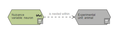
For example, in an experiment investigating the effect of a systemic drug on the response of individual neurons, the experimental unit is the animal even though multiple neurons are recorded from each animal. In this case the individual neurons are nested within the individual animal. The analysis should be carried out using one measurement per animal, rather than using the data from each neuron measured as independent data points. To achieve this the data from individual neurons from the same individual should be averaged for each animal before running the statistical analysis.

In general, it is recommended to always average up to the experimental unit level. This approach reduces the between-animal variability as the multiple replicates measured per animal are used to produce a more precise single measurement. The exception to this general rule would be a specialist analysis to investigate the variability associated with the multiple nested variables, or a situation where the responses are measured over time and are analysed using a repeated measures approach.

Back to top

Using covariates

The variability associated with a continuous nuisance variable can be accounted for by including it as a covariate in the statistical analysis.

There may be a baseline measurement that has a strong relationship with the response of an animal to a treatment, and some of the post-intervention variability in the response can be explained by accounting for the variability in the baseline measurements. 

Using a variable as a covariate captures background information that may influence and explain post-experimental differences between individual experimental units. Consider doing this to deal with the influence of a continuous nuisance variable that is not readily controllable. Examples of variables that can be used as covariates include a pre-treatment measure of the response of interest, baseline bodyweight or age of the animal. These values should ideally be measured before the animal undergoes any intervention that corresponds to an independent variable of interest. 

Consider an example of an experiment to examine the effect of a novel compound on locomotor activity. The more active animals before treatment are likely to be the more active animals at the end of the study, regardless of the treatment they received. Using baseline locomotor activity as a covariate takes this into account and reduces the overall between-animal variability after treatment. This increases the statistical power of the test to detect the effect of the compound.

Back to top

How to check if including a covariate is appropriate

To decide if a covariate should be included in the statistical analysis check that it meets these three assumptions:

1. There is a linear relationship between the outcome measure and the covariate. 
2. The relationship between the outcome measure and the covariate is similar for all treatments.
3. The covariate is independent of treatment.

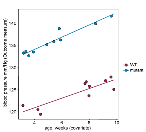
These assumptions can be explored by plotting the data, for example using a categorised scatterplot. Plot the primary outcome measure against the covariate, colour coded by the treatment groups, as seen in the examples below. These graphs are adapted from output automatically generated in InVivoStat when a covariate is included in the statistical analysis.

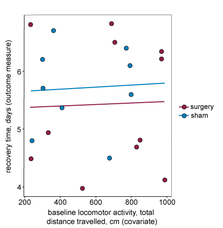
Assumption one – There is a strong relationship between the outcome measure and the covariate.

For the first assumption to hold, the covariate should explain some of the variability in the outcome measure. This happens when the outcome measure and the covariate are correlated. In the graph below, the regression lines on the plot are almost horizontal, indicating that there is a weak relationship between the covariate and the outcome measure. If the covariate is included in the statistical analysis it will not explain enough of the variability in the outcome measure to justify its inclusion, reduces the power of the experiment by using a degree of freedom to estimate the linear relationship. We do not recommend including this covariate in the analysis.

 

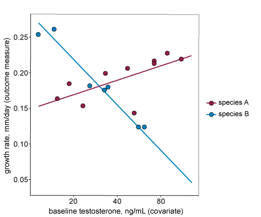
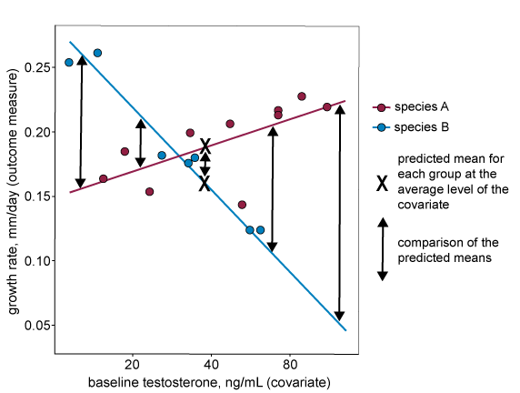
Assumption two – The linear relationship between the outcome measure and the covariate is similar for all treatments.

For the second assumption to hold, the covariate should have the same effect in all treatment groups (i.e. the relationship between the outcome measure and the covariate is the same for all treatment groups). In the graph below, the regression lines (each representing a separate treatment group, in this case a different species) are not parallel. This indicates that the relationship between the outcome measure and the covariate is different for each treatment group. We do not recommend including this covariate in the analysis.

 

 Assumption three – The covariate is independent of treatment.

For the third assumption to hold, the covariate values should not be different across the groups in the analysis. If the values are different then this is defined as a confounding covariate.

In the graph below, data from the drug and control groups are separated along the x-axis (bodyweight). This indicates that the covariate is different in the drug treated group and the control group and therefore the covariate is not independent of the treatment and is a confounding variable. In these situations, including the covariate is risky because in the process of fitting a common regression line you may remove part of the treatment effect. This leads to false negatives.

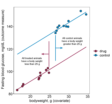
In cases where the intervention is something the researcher can assign to animals (e.g. a drug or surgical intervention) the covariate can be balanced across groups by appropriate randomisation strategies (e.g. using bodyweight, such as high and low weight, as a blocking factor in the randomisation or by using minimisation randomisation). This will ensure assumption three holds and removes the potential risk if the assumption is not met.

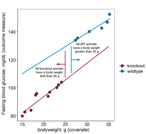
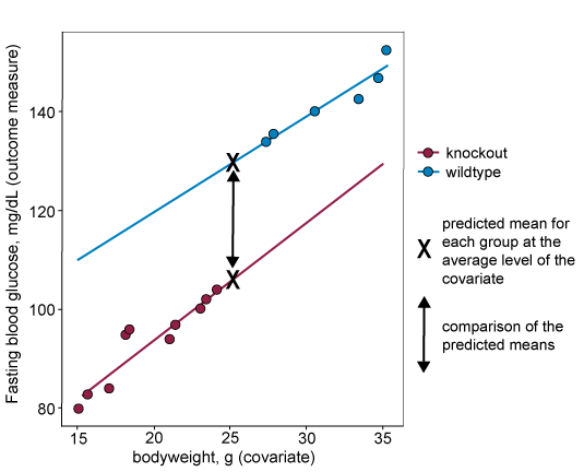
But what if the intervention is something the researcher cannot assign to animals (e.g. genotype)? The graph below shows data from wildtype and knockout groups where the covariate (bodyweight) does not overlap along the x-axis. This indicates that the covariate is different in the wildtypes and the knockouts and therefore the covariate is not independent of the intervention. The covariate is a confounding variable. In fact, as body weight is a highly heritable trait it is commonly altered in knockout lines of mice. This introduces challenges as body weight correlates with many other biologically interesting variables (e.g. heart weight, grip strength). If this confounding variable is included as a covariate in the analysis it changes the research question to ‘What is the effect of the intervention after adjusting for any body weight differences?’ in other words is there still a difference in the outcome measure for the different interventions after accounting for the difference in body weight? This can only be answered by the inclusion of body weight as a covariate. The analysis can be conducted including the covariate provided the visual inspection of the data suggests a common linear relationship would be appropriate (i.e. the linear lines on the plot are parallel), but it does have implications for the study conclusions. 

When to include a covariate in the analysis

In the example below all three assumptions hold and the covariate can be included in the analysis:

1. The response and covariates are positively correlated – the covariate does explain the between animal variability in the response and is worth including in the statistical analysis (i.e. including it will not reduce power).
2. The regression lines on the plot are parallel – the response/covariate relationships are similar across the two treatment groups.
3. There is no treatment effect of the covariate – there is a horizontal overlap between the two treatment groups along the x-axis.

In many cases you will not know if including a particular covariate in the analysis is appropriate when planning an experiment. In these cases, measure the covariate during the study, but only include it in your statistical analysis if the assumptions for covariate inclusion are met.

Back to top

Why it is important that the assumptions for covariate inclusion hold

When including a covariate in a statistical analysis, such as ANCOVA, group means used in the analysis are adjusted to correspond to what the mean would be for each group at the overall average of the covariate. A mean adjusted in this way if often called the 'predicted mean'. Groups are then compared using the predicted mean for each group, see the 'X's in the graph below. For this approach to generate reliable 'predicted means', and reliable comparisons between the means, the assumptions described in the section above must hold.

 

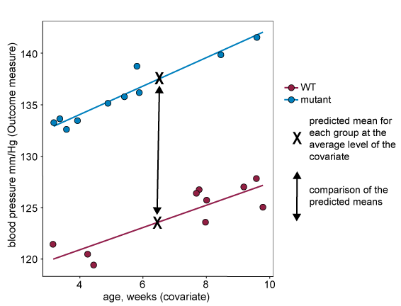
 When the data violates assumption two (if the regression lines are not parallel), the size of the difference between predicted means will depend on the level of the covariate where the comparison is made. This is shown on the graph below, where the difference between predicted means in the analysis (marked with an X on the graph) will be very small despite the fact that there is evidence of the intervention having a large effect at more extreme levels of the covariate.

 

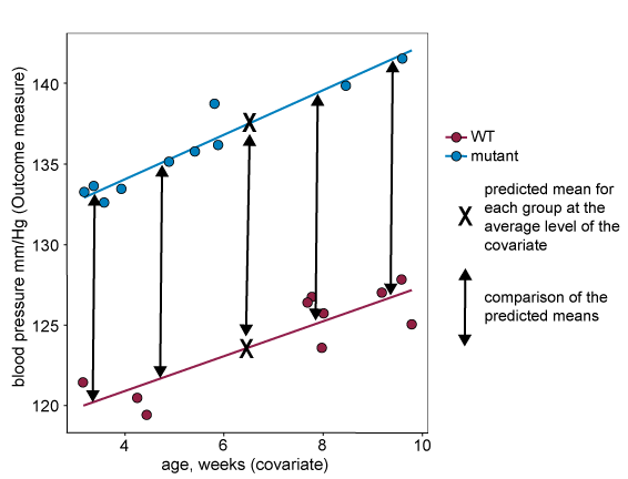
If the lines are parallel and assumption two holds, then the size of the difference between predicted means is independent of where along the covariate the comparison is made. You can see on the graph below that the size of the difference is the same regardless of covariate level. This means that the difference between predicted means is a reliable estimate of the treatment effect.

 For data that does not fit assumption three, the covariate levels are systematically different across the treatment groups. This means that the predicted mean at the overall average level of the of the covariate can be misleading and not reflect the actual data. In the example below for which assumption three does not hold, the predicted mean for the knockout group is higher than all actual responses from that group. 

In some cases, including the example above, there is confounding you cannot do anything about. The section below discusses the implications of including a confounding covariate in your analysis

Back to top

What if the covariate is not independent of the treatment?

Including a confounding covariate to take account of some variability can give biological insights and is a much more robust method than normalising groups using a ratio correction. However, it is important to know that by including a confounding covariate you are making more assumptions. For example, as well as assuming a linear relationship between the confounding variable and the variable of interest you are also assuming that the predicted response, at the average value of the covariate (or the extrapolation to the average covariate, as in the plot below) is reliable and meaningful. 

Additionally, you risk removing some of the effect of the intervention (e.g. genotype in the example below) while accounting for the effect of the covariate (e.g. bodyweight in the example below). This means you are more likely to get a false negative. in reality you are also asking a slightly different research question when including a confounding covariate compared to a non-confounding covariate (i.e. you are changing your hypothesis). In the example below you are asking, is there a fundamental difference in blood glucose? (yes or no) but also is some of that difference accounted for by the body weight difference? (yes or no). 

Uncontrolled variable

In some instances you may not be able to control for a nuisance variable. 

One example could be an experiment comparing measurements from wild type and mutant litters. If only a limited number of animals can be obtained at any one time, then the day of measurement would be a nuisance variable. Ideally, the ‘day’ nuisance variable would be used as a blocking factor to ensure an equal number of measurements from mutant and wild type animals are made on each day. However, if the litters are born at different times and animals from the two genotypes cannot be recorded on the same day then ‘day’ cannot be used as a blocking factor. In this case it is not possible to avoid confounding the nuisance variable ‘day’ with the independent variable of interest ‘genotype’ and the ‘day’ variable remains uncontrolled. 

The only protection against such nuisance variables is adequate replication. With enough repeats, the randomisation strategy makes it unlikely that the nuisance variable is confounded with the independent variable of interest. If adequate replication is not possible, such that a confound remains, then the experiment may not be worth carrying out.

Back to top

Continuous and categorical variables

Variables can be categorical or continuous:

Continuous variables include truly continuous variables but also discrete variables. Levels consist of numerical values, for example bodyweight, age, time to event. 

Categorical variables have levels that are non-numeric, for example sex (categories: ‘male’ and ‘female’). Categorical variables can be ordinal, nominal or binary.

Some variables can be considered as either. For example drug dose (levels: ‘vehicle’, ‘low’ and ‘high’ dose, if it is categorical, or levels: 0, 1 and 10, if it is continuous) or time can be considered continuous or distinct time points (levels: ‘pre-intervention’ and ‘post-intervention’). Deciding whether to treat these variables as continuous or as categorical depends on the objective of the experiment. 

For example treating drug dose as a continuous variable enables modelling of the dose-effect relationship, perhaps with a curve or regression line, and the underlying relationship between dose and effect can be estimated. The analysis provides an estimate of the relationship – it will not test a hypothesis but can identify the dose that causes a biologically relevant effect (which might not be one of the doses assessed).

Treating drug dose as a categorical factor enables a comparison between the individual treatment group means and a test of the null hypothesis (H0) that there is no difference between the groups treated with vehicle, low and high doses.

This choice impacts on the experimental design. If drug dose is treated as categorical the experimental design should include a limited number of dose groups, but each group should contain sufficient animals to power the pairwise tests. If drug dose is treated as continuous it would be best to include more doses in the design, with fewer animals at each dose.

For nuisance variables, treating a variable as continuous or categorical depends on how the variability is accounted for. Categorical variables can be used as blocking factors and continuous variables can be used as covariates. If a nuisance variable can be considered as either, it can be used differently in the allocation and the analysis. For example, bodyweight can be considered categorical and used as a blocking factor in the allocation (categories: 'low weight' and 'high weight') and as a continuous covariate in the analysis.

Back to top

Allocation of experimental units into the categories of a variable

Experimental units are allocated to the different categories (or levels) of a particular variable, to test the effect of a variable of interest or to control the effect of a nuisance variable. This allocation should be random (see randomisation section) and in most cases, it will be possible to randomise experimental units to an independent variable’s categories. 

For some variables, for example animal characteristics such as sex or genotype, even though the randomisation is not done by the experimenter it can be assumed that animals have been allocated into categories (such as male or female, or a particular genotype) at random, via Mendelian inheritance.

However, for other variables, it is not possible to allocate experimental units at random. In these cases it is important to realise that, because allocation has not been random, it is impossible to conclude that any relationship is causal. Nonetheless, it may be a useful predictor of the response.

For example, in an experiment where bodyweight is used as a blocking factor, animals cannot be randomised into weight ranges as they are allocated to different categories of that nuisance variable based on their bodyweight. It is impossible for a researcher to conclude that body mass, rather than something correlated with body mass, causes a difference in response.

Back to top

Repeated factor

A repeated factor is an independent variable of interest which is shared across all animals in the experiment and cannot be randomised.

In a situation where you measure animals (or experimental units) repeatedly over time, and time is an independent variable of interest, then ‘time’ is a repeated factor. Note the levels of a repeated factor cannot be randomised – ‘day 1’ must come before ‘day 2’.

There are two situations where including a repeated factor of interest (also known as within subject factor) would be appropriate: in repeated measure designs and dose escalation designs. 

The crucial difference between a repeated measure and dose escalation design is that in a repeated measure design the experimental unit is usually the animal (which is then measured repeatedly), whereas in the dose-escalation design the experimental unit is the animal within a time period (so each experimental unit is measured only once).

In a repeated measure design, measurements are taken from each animal or experimental unit in a non-random order. For example, the animals are measured at specific time points or in specific brain regions which cannot be randomised (t0 always comes before t1, brain is scanned front to back). The repeated factor would then be ‘timing of measurement’ or ‘brain region’ and all animals are measured across all categories of these variables. 

In a dose-escalation design, animals receive multiple treatments (and measurements) over time in a non-random order, for example escalating doses of a drug to avoid toxicological effects. The variables ‘drug’ and ‘timing of measurement’ are combined because all animals get the same dose at the same time. The repeated factor would then be ‘drug’ and all animals are measured across all categories (drug doses). 

If the order of the repeated measurements can be randomised, it would not be appropriate to include the variable which relates to the timing of measurement or the test period as a repeated factor in the analysis. In a crossover design for example, where each animal receives multiple treatments in a random order and each animal is used as its own control, 'timing of measurement' would be a blocking factor for the analysis.

Back to top

Representing independent variables in the EDA

The EDA will provide tailored advice and feedback through the critique function to help you build your experiment diagram and identify and characterise your variables. 

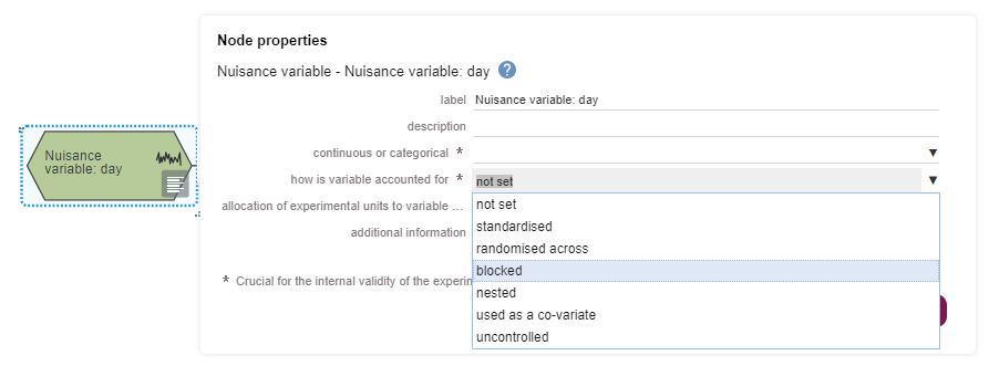
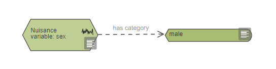
Your EDA diagram uses different nodes for independent variables of interest and nuisance variables. Variables can be categorical or continuous – you can indicate this in the properties of the variable node. If a variable is categorical, you should link category nodes, defining the levels of the factor, to the variable node. In the properties of the independent variable nodes, the field 'categorical or continuous' relates to how the variable is treated in the analysis.  

For the variables of interest, variable categories nodes are used as ‘tags’ on the diagram. Variable categories can be tagged to three different types of nodes:

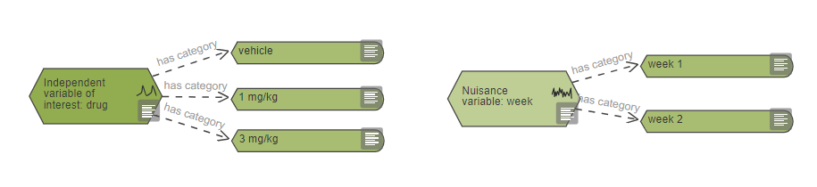
• Intervention nodes – for example when the independent variable is treatment, such as in Example 1.The independent variable of interest ‘Drug A’ has two categories: ‘vehicle’ and ‘drug’. These variable categories are used to tag the two intervention nodes to indicate the treatment each group of mice receives.
• Group nodes – for example when the independent variable is an animal characteristic such as ‘sex’ in Example 3. The two categories ‘male’ and ‘female’ are tagged to the groups to indicate the composition of each experimental group.
• Measurement nodes – for example when the independent variable relates to a timing such as ‘time of measurement' in Example 3. Each time point is represented as a category node and tagged to the relevant measurement nodes.

For clarity, several instances of the same variable categories can be included on the diagram. In Example 1, the two category nodes have been duplicated to prevent arrows running across the diagram. The system considers nodes with the same labels to be several instances of the same category. Similarly, in Example 2 the nuisance variables ‘test period’ and ‘animal’ each appear twice on the diagram. Only one instance of each variable has to have full information. If multiple nodes exist for the same variable, the variable should be defined using the node that is connected to the analysis – categories should be connected to this node and relevant information should be provided in its properties. This is to enable the EDA to provide recommendations regarding appropriate statistical analysis methods.

Independent variables can be categorical or continuous, this must be indicated in the properties of the variable node so that the system can make an accurate analysis recommendation. 

Experimental units are allocated to the different categories of variables. In your EDA diagram, you can indicate how the experiments units are allocated to categories for all independent variables of interest and nuisance variables, in the properties of the variable nodes.

Back to top

Representing independent variables of interest in the EDA​

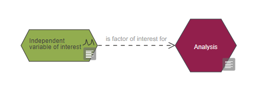
To indicate that an independent variable of interest is a factor of interest in an analysis, connect the nodes as shown:

Often, an experiment has several variables of interest. Each should have its own independent variable of interest node:

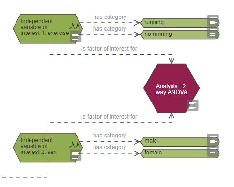
The example above is an experiment looking at the effect of exercise on neuronal density. There are two variables of interest:

• Exercise with two categories: 'running' and 'no running' – animals are randomised by the investigator into one of these two categories to test the effect of exercise on neuronal density.
• Sex with two categories: male or female – to check whether the effect of exercise differs between males and females.

It is important to identify repeated factors correctly in an EDA diagram as this has implications for the analysis. Whether a variable of interest is a repeated factor can be indicated in the properties of the variable node.

Back to top

Representing nuisance variables in the EDA

Nuisance variables are other sources of variability or conditions which may influence the outcome measure and are indicated on your EDA diagram using nuisance variable nodes. Depending on the type of nuisance variable and the objective of your experiment, there are different ways to account for the variability.

Nuisance variables could be:

• Standardised
• Randomised
• Blocked
• Nested within another variable
• Used as a covariate 

If none of these are done, then the variable is uncontrolled. This information should be provided in the properties of the nuisance variable nodes.

In your EDA diagram, standardised nuisance variables are represented with only one category. They are not connected to the rest of the diagram because once standardised they do not add variability to the experiment. Standardising nuisance variables will limit how far the conclusions of your experiment can be generalised.

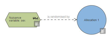
To indicate that a nuisance variable is accounted for by randomisation, it should be connected to the allocation node with a link 'is randomised by'.

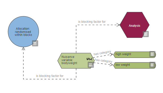
To show that a nuisance variable is a blocking factor in the randomisation, it should be connected to the allocation with the link ‘is blocking factor for’. Depending on your experimental design the nuisance variable could be included in the analysis as either a covariate (using the link ‘is covariate for’) or as a blocking factor as shown in the image below (using the link ‘is blocking factor for’).  For more information on randomisation with blocking factors go to the allocation section. 

 A nested nuisance variable is indicated by connecting it to the variable it is nested within. Nested variables can be linked to any other variable and also the experimental unit node.

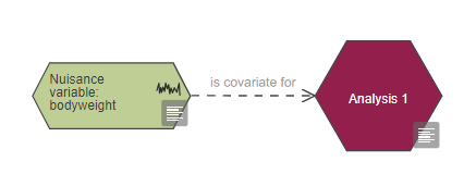
 To show that a nuisance variable will be used as a covariate connect it to the analysis node with the link 'is covariate for'.

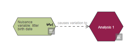
 Any uncontrolled nuisance variables should be flagged as uncontrolled in your EDA diagram and should be connected with a link to the measurement and the analysis nodes using the link 'causes variation to'. 

Back to top​

References

Altman, DG and Bland, JM (2005). Treatment allocation by minimisation. BMJ 330(7495):843. doi: 10.1136/bmj.330.7495.843
Bate, ST and Clark, RA (2014). The Design and Statistical Analysis of Animal Experiments. Cambridge University Press.
Dayton, CM (2005). Nuisance Variables. In: Encyclopedia of Statistics in Behavioral Science (Eds. Everitt, B and Howell, D). John Wiley & Sons, Ltd.
Dean, AM and Voss, D (1999). Design and Analysis of Experiments. Springer-Verlag.
Festing, MFW, et al. (2002). The design of animal experiments: reducing the use of animals in research through better experimental design. Royal Society of Medicine.
Gaines Das, RE (2002). Role of ancillary variables in the design, analysis, and interpretation of animal experiments. ILAR J 43(4):214-22. doi: 10.1093/ilar.43.4.214
Karp, NA, et al. (2012). The fallacy of ratio correction to address confounding factors. Lab Anim 46(3):245-52. doi: 10.1258/la.2012.012003
Kirk, RE (2009). Experimental Desgin. In: The SAGE Handbook of Quantitative Methods in Psychology (Eds. Maydeu-Olivares, A and Millsap, RE). Sage.
Lazic, SE (2010). The problem of pseudoreplication in neuroscientific studies: is it affecting your analysis? BMC Neurosci 11:5. doi: 10.1186/1471-2202-11-5
Reed, DR, et al. (2008). Reduced body weight is a common effect of gene knockout in mice. BMC Genet 9:4. doi: 10.1186/1471-2156-9-4