Analysis

How to choose a method of analysis, and test and transform data to meet the assumptions of parametric tests.

Contents

• Choosing a method of analysis
• Parametric and non-parametric tests
  • Normal distribution
  • Homogeneity of variance
• Data transformation
  • Log_e and log₁₀ transformation
  • Square root transformation
  • Arcsine transformation
  • Rank transformation
• Multiple testing corrections
• Post-hoc testing
  • Tests adjusted for multiple comparisons
    • Dunnett test
    • Tukey HSD
    • Bonferroni
    • Step-wise tests
  • Unadjusted tests
    • Fisher’s LSD
• Number of factors of interest
• Analysis method suggestions from the EDA
• Representing analysis plans in the EDA
• Representing data transformation in the EDA

In comparative experiments, statistical analysis is used to estimate effect size and determine the weight of evidence against the null hypothesis.

Choosing a method of analysis

Statistical analysis strategies should be chosen carefully to ensure that you can draw valid conclusions from your data. Which test is appropriate depends on the number of outcome measures, the properties of these outcome measures, the independent variables of interest and whether any additional sources of variability (i.e. nuisance variables) need to be accounted for. It also depends on whether the data collected satisfies the parametric assumptions. 

Back to top

Parametric and non-parametric tests

Parametric tests have more statistical power than non-parametric tests, as long as the parametric assumptions are met. When the data does not satisfy these assumptions, non-parametric tests are more powerful. However, in many cases the parametric assumptions can be satisfied by using a data transformation. This should be attempted before considering a non-parametric method of data analysis.

When assessing the assumptions, you must consider the residuals of the analysis, as well as the data itself. The ‘residual’ is the difference between the observation and its prediction. The ‘predicted value’ is the value predicted by fitting the statistical model to the data (for example a group mean). 

Data are suited to parametric analysis if they satisfy the following assumptions: 

• The data is continuous, rather than categorical or binary.
• The responses are independent (i.e. each observation should not be influenced by any other, once all sources of variability are accounted for). 
• The residuals from the analysis are normally distributed.
• The different groups have similar variances (the homogeneity of variance assumption).

Back to top

Normal distribution

Parametric tests, such as the t-test, ANOVA and ANCOVA, carry the assumption that your responses, or more precisely the residuals from the analysis, are approximately normally distributed. Many biological responses follow this distribution. If a response that is normally distributed is measured repeatedly, under the same experimental conditions, you would expect most of the responses to lie close to the centre of the distribution, with increasingly fewer responses observed as you move away from the centre. There will be approximately the same number of responses observed above the centre as below it, giving a symmetric distribution.

There are various tests for normality, including the Shapiro-Wilk and Kolmogorov-Smirnov tests. However, these tests struggle to detect non-normality if the sample size is small, as is often the case with animal experiments. An alternative approach is to produce a normal probability plot, where the observed residuals are plotted against the predicted residuals if the data was normally distributed. If the points on the plot lie along a straight line, then this is a good indication that the normality assumption holds.

Back to top

Homogeneity of variance

One of the key assumptions of most parametric tests is that the variance in all groups is about the same. This implies that the variability of the response is not dependent on the size of the response. For example, the within-group variability does not depend on the size of the group mean. This is because the null hypothesis being tested is that the groups are samples from the same population and so any differences in the means, or variances, are due to chance.
 
With biological responses, the variability often increases in magnitude as the response increases. This increases the risk that assumption of homogeneity of variance may not hold.

There are several tests you can use to assess the homogeneity of variance, including the Brown-Forsythe test and Levene’s test. However, as with the formal tests of normality these are not recommended when the sample size is small, as is often the case with animal experiments. An alternative approach is to produce a residual vs predicted plot. If the scatter of points on this plot is random, with no patterns such as a fanning effect (indicating the residuals get larger as the predicted values increase) then the homogeneity of variance assumption holds.

Back to top

Data transformation

If your data are not normally distributed and/or the homogeneity of variance assumption does not hold, a data transformation can help you satisfy the parametric assumptions and enable you to use the more sensitive parametric tests. 

Data transformation involves replacing the variable with a function of that variable. Common transformations include ‘mathematical’ transformations (e.g. log, square root or arcsine) or the rank transformation.

Log_e and log₁₀ transformation

Log transformations are useful when a response increases exponentially (for example bacterial cell counts). It is perhaps the most common transformation applied to biological data and involves taking the log value of each observation. This can be performed on either the log₁₀ or log_e scale. 

One disadvantage of applying a log transformation is that zero or negative responses cannot be transformed. If the outcome measure being analysed contains zero or negative values, you must add a small offset onto all responses so that all data are positive.

Square root transformation 

Square root transformation involves taking the square root of each response. Similarly to log transformations, a square root transformation cannot be applied to negative numbers. To overcome this, if any responses are negative, you must add a constant to all numbers to use the square root transformation.

We recommend the square root transformation prior to analysis of count response data.

Arcsine transformation

Arcsine transformation consists of taking the arcsine of the square root of a number. An arcsine transformation may be appropriate for proportion responses, which are bounded above by 1 and below by 0. 

When responses are bounded above and below, there is a tendency for the variability of the response to decrease as it approaches these boundaries. The arcsine transformation effectively increases the variability of the responses at the boundaries and decreases the variability of the responses in the middle of the range.

You can transform any response that is bounded above and below using this method, but if the responses are not contained within the range of 0 to 1, you will need to scale the responses to fit this range first.

Rank transformation

If, even after a mathematical transformation, the parametric assumptions do not hold, a rank transformation can be used. You can then apply parametric tests to the rank transformed data.

A rank transformation consists of ranking the responses in order of size, with the largest observation given the rank 1, the second largest, rank 2, and so on. 

Note that rank transforming the data loses information and potentially reduces the power of the experiment. The ranking technique also implies that the results of the statistical analysis are less likely to be influenced by any outliers. For example, on the original scale, the largest observation in the dataset may appear to be an outlier, but it is given rank 1 regardless of the actual numerical value. This observation will be given the same rank regardless of how extreme it is.

Back to top

Multiple testing corrections

In many biology-related fields it is relatively common to test multiple hypotheses and hence make multiple comparisons in a single experiment. For example, if several behaviours are measured, or in high throughput or ‘-omics’ experiments. In such situations, it is important to correct for random events that falsely appear to be significant.

In an experiment with one hypothesis, a significance level (α) set at 0.05 means that when the null hypothesis is true the probability of obtaining a true negative result is 95% and the probability of obtaining a significant result by chance (a false positive) is 5% (1 – 0.95). This ‘false positive’ probability increases exponentially with multiple hypotheses.
 
With the same significance level, for an experiment with three hypotheses the probability of obtaining a false positive result is raised to 14% (1 – 0.953), with 25 hypotheses it is raised to 72% (1 – 0.9525), and with 50 hypotheses there is a 92% chance of obtaining a false positive (1 – 0.9550). The aim of multiple comparison procedures is to reduce this probability back down to 5%. See the Bonferroni correction described below.
 

Back to top

Post-hoc testing

If you analyse your experiment using an ANOVA approach and the null hypothesis is rejected, this implies that there is a difference among the group means but it does not indicate which groups are different. To determine which groups are different you can perform subsequent post-hoc testing.
 
There are several post-hoc tests to choose from, depending on if you planned the post-hoc comparisons in advance and whether all-pairwise comparisons, or only comparisons with the control group are required. You should only run one post-hoc test per experiment.

Tests adjusted for multiple comparisons

Dunnett test

The Dunnett test is a good choice when comparing groups against a control group and it provides a correction for multiple comparisons, thus reducing the likelihood of false positive conclusions (type 1 error).

Tukey HSD (honest significant difference)

The Tukey HSD test essentially compares everything with everything. It calculates all possible pairwise comparisons and provides adequate compensation for multiple comparisons. However, if you are only making some pairwise comparisons, this post-hoc test is overly strict and therefore increases the likelihood of false negative conclusions (type 2 error).

Bonferroni test

The Bonferroni test can be used for planned comparisons between a subset of groups, and concurrently adjusts the significance levels to account for multiple comparisons. 

To perform the Bonferroni correction, the significance level is readjusted by dividing it by the number of comparisons. So for three comparisons, the significance cut-off point is set at 0.017 (α/n = 0.05/3), and for 25 comparisons, it is set at 0.002 (α/n = 0.05/25). This correction is simple to perform but very conservative – it greatly reduces the risk of obtaining false positives but increases the risk of obtaining false negatives when dealing with large numbers of comparisons.
 

Step-wise tests

Alongside the tests above, all of which apply a single adjustment to all tests simultaneously, there are also tests that apply adjustments in a step-wise manner, for example the Hochberg, Hommel and Holm tests. These tests have been shown to be powerful alternatives to the more traditional approaches.

Unadjusted tests

Fisher’s LSD (least significant difference)

The LSD test is considered to be a more reliable test than simply performing lots of separate t-tests. The test performs a series of t-tests among selected pairs of means, and the variability estimate used in all calculations is the more reproducible estimate taken from the ANOVA table (the Mean Square Error). However, it does not correct for multiple comparisons and so it is more likely to detect differences which are not real (type 1 ‘false positive’ error).

Back to top

Number of factors of interest

If you have many different independent variables which may or may not influence the response, you can assess them all in one factorial experiment.

Running several experiments, where a single factor of interest is varied in each, might not make the most efficient use of the animals and does not allow you to see if there are any interactions between the factors. In addition, modelling a condition often requires more than just one factor to explain changes in the outcome measure. You can use factorial designs to test the effect of multiple factors simultaneously. 

Factorial designs can be used to assess which levels of the independent variables of interest (such as treatment formulation and dose) should be selected to maximise the ‘window of opportunity’ to observe a treatment effect. When setting up a new animal model, while it may seem a waste of resources to run such pilot studies at the start of the experimental process, the long-term benefits can easily outweigh the initial costs.

As an example, consider a study conducted to assess the response to a drug with different formulations. This experiment would allow the scientist to select the formulation that was most sensitive so that future experiments would have the largest window of opportunity to capture a treatment effect of similar novel compounds. This allows a reduction in the number of animals required to test the novel compounds. 

Bate and Clark (2014) differentiate between two types of factorial design –  large and small.

‘Large’ factorial designs are used to investigate the effect of many factors and how they interact with each other. You may also want to identify factors that can be ignored as having no significant effect on the response. These designs are particularly useful, for example, when setting up a new animal model. Large factorial designs necessarily involve many individual groups but because you are only interested in the overall effects, and do not need to make pairwise comparisons between the groups, the individual sample sizes can be small.

‘Small’ factorial designs, which are commonly applied in animal research, consist of usually no more than two or three factors. The purpose is to compare one group mean to another, using a suitable statistical test. It is important these types of experiments are adequately powered (with suitable sample sizes in each group) to allow pairwise comparisons between the combinations of factors.
 

Back to top

 Analysis method suggestions from the EDA

Once the EDA diagram is complete and any feedback from the critique has been dealt with, the EDA can generate a suggestion of statistical tests which are compatible with the design of the experiment. At this stage, the system has no information on whether the data satisfies the parametric assumptions and so the EDA recommends both a parametric and a non-parametric method. You will need to assess these assumptions when you have your data in order to choose which method to use.

Once the EDA has suggested an analysis method, but before you start your experiment, indicate your planned method of analysis for each of the analysis nodes on your EDA diagram. Once your data are collected, there is sometimes a rationale to deviate from the planned method. For example, if the data does not satisfy the parametric assumptions and data transformation fails to address this, a non-parametric analysis method may be more appropriate. You can update your diagram for reflect this and indicate the method of analysis used, along with the reason for not using the planned method.

Regardless of whether your data satisfy parametric assumptions, how these assumptions are assessed should be indicated in the properties of the analysis node.

Back to top

Representing analysis plans in the EDA

In your EDA diagram, an analysis node should receive input from at least one outcome measure and be connected to at least one variable of interest.

If nuisance variables are included in the analysis, for example as blocking factors or covariates, then they should also be connected to the analysis node, using the appropriate link.

In a situation where only a subset of the recorded data is included in the analysis, the variable category (and not the variable itself) should be connected directly to the analysis node. This indicates that the analysis is only conducted on the data from that category. For example, if responses were measured at several time points but for one analysis only data from one specific time point is used (see analysis 2 in the example below). 

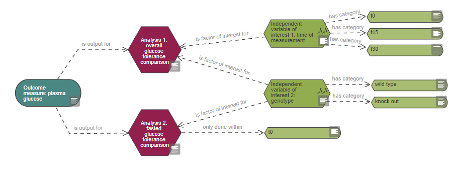
Information captured in the analysis node includes:

• The method of analysis you plan to use.
• Whether you plan to use a post-hoc test.
• Whether you will use multiple testing corrections.
• Whether the analysis will be conducted blind (see blinding section).
• If blinding will not be used, specify the reason why.

If multiple analyses are performed on the experimental data, one analysis node per analysis should be included on the diagram. The primary analysis, which is used to calculate the sample size should be identified.

Back to top

 Representing data transformation in the EDA

See the measurement section for how to represent data transformation in your EDA diagram.

Back to top

References

Altman, DG and Bland, JM (2009). Parametric v non-parametric methods for data analysis. BMJ 338. doi: 10.1136/bmj.a3167
Bate, ST and Clark, RA (2014). The Design and Statistical Analysis of Animal Experiments. Cambridge University Press.
Bland, JM and Altman, DG (1996). Statistics notes: Transforming data. BMJ 312(7033):770. doi: 10.1136/bmj.312.7033.770
Conover, WJ and Iman, RL (1981). Rank transformations as a bridge between parametric and nonparametric statistics. The American Statistician 35(3):124-129. doi: 10.2307/2683975
Festing, MF and Altman, DG (2002). Guidelines for the design and statistical analysis of experiments using laboratory animals. ILAR J 43(4):244-58. doi: 10.1093/ilar.43.4.244
Marino, MJ (2014). The use and misuse of statistical methodologies in pharmacology research. Biochem Pharmacol 87(1):78-92. doi: 10.1016/j.bcp.2013.05.017
Nakagawa, S and Cuthill, IC (2007). Effect size, confidence interval and statistical significance: a practical guide for biologists. Biol Rev Camb Philos Soc 82(4):591-605. doi: 10.1111/j.1469-185X.2007.00027.x