Group and sample size
How to define the experimental groups and calculate the sample size needed to obtain reliable results.
- Defining experimental groups
- Sample size
- Why power analysis is important
- Choosing the appropriate power calculation
- Calculate your sample size
- Parameters in a power analysis for t-tests
- Representing groups in the EDA
- Indicating sample size in an EDA diagram
Defining experimental groups
Every experiment you conduct should include at least one control or comparator group. Controls can be negative controls, typically animals receiving a placebo or sham treatment, or sometimes untreated animals. Positive controls may be included to check that an expected effect can be detected in the experimental settings.
The choice of control or comparator group depends on the objective of your experiment. Sometimes a separate ‘no treatment’ control may not be needed. For example, if the aim of your experiment is to compare a treatment administrated by different methods (e.g. intraperitoneal administration or oral gavage), a third group with no treatment is unnecessary.
Typically experiments also include a group receiving an intervention that is being tested. For example, if your study compares the effect of a drug vs a control substance on blood glucose levels, one group would receive the drug/intervention and the other would receive the control.
Sample size
Sample size is the number of experimental units per group
If the experimental unit is the individual animal, your sample size will be the number of animals per group. If the experimental unit comprises multiple animals (for example, a cage or a litter – see the experimental unit section for additional examples), the sample size is less than the number of animals per treatment group.
If your experiment is designed to test a formal hypothesis using inferential statistics and the generation of a p-value, you should determine the number of experimental units per group using an appropriate method such as a power analysis. Basing your sample sizes solely on historical precedent should be avoided. This can lead to wastage of animals via either an underestimation of animals required (meaning you are unable to draw significant conclusions from your study) or in a serious overestimation of sample size needed.
If you are replicating another study that was 'only just' statistically significant, your replication has at least a 50% chance of failure if you use the same sample size as in the original study (see Button et al., 2013).
If your experiment is not intended to test a formal hypothesis, power calculations are not appropriate and sample sizes can be estimated based on experience, depending on the goal of the experiment.
This type of experiment includes:
- Preliminary experiments testing for adverse effects.
- Preliminary experiments checking for technical issues.
- Experiments, such as the production of antibodies or a transgenic line, which are based on success or failure.
If your preliminary study is large enough (e.g. as rule of thumb 10 animals or more per group), variability data collected in these experiments can also help you calculate the sample size needed in follow up studies designed and powered to test some of the hypotheses they generate. However, systematic reviews and previous studies are usually a more appropriate source of information on variability.
Using a balanced design, in which all experimental groups have equal size, maximises sensitivity in most cases. Examples of where balanced studies usually maximise sensitivity include those involving only two groups, or several groups where all pairwise comparisons will be made. For some experiments however, sensitivity can be increased by putting more animals in the control group – for example those involving planned comparison of several treatment groups back to a common control group.
Why power analysis is important
In a hypothesis-testing experiment you usually take samples from a population, rather than testing the entire population. If you observe a difference between the treatment groups, you need to determine whether that difference is due to a sampling effect or a real treatment effect.
An appropriate statistical test manages the sampling issue and calculates a p-value to help you make an informed decision. The p-value is the chance of obtaining results as extreme as, or even more extreme than, those observed if the null hypothesis is true.
The smaller the p-value, the more unlikely it is that you could obtain the observed data if the null hypothesis were true and there was no treatment effect. A threshold (α) is set, and by convention a p-value below the threshold is deemed statistically significant. This means that the result is sufficiently unlikely that you can conclude that the null hypothesis is not true and accept the alternative hypothesis. The table below describes the possible outcomes when using a statistical test to assess whether to accept or reject a null hypothesis.
| No biologically relevant effect | Biologically relevant effect | |
| Statistically significant p < threshold (α) H0 unlikely to be true |
False positive Type 1 error (α) |
Correct acceptance of H1 Power (1-β) |
| Statistically not significant p > threshold (α) H0 likely to be true |
Correct rejection of H1 | False negative Type 2 error (β) |
A power calculation is an approach to assess the risk of making a false negative call (i.e. thinking your results are not significant when they are). The power (1-β) is the probability that your experiment will correctly lead to the rejection of a false null hypothesis. Another way of putting it is that the power is the probability of achieving statistically significant results when there actually is a biologically relevant effect.
The significance threshold (α) is the probability of obtaining a significant result by chance (a false positive) when the null hypothesis is true. When set at 0.05, it means that the risk of obtaining a false positive is 1 in 20, or 5%.
Under-powered in vivo experiments waste time and resources, lead to unnecessary animal suffering and result in erroneous biological conclusions.
The smaller the sample size the lower the statistical power – there is little value in running an experiment with too few samples and a low power. For example, with a power of 10% the probability of obtaining a false negative result is 90%. In other words, it is very difficult to prove the existence of a ‘true’ effect when too few animals are used.
In addition, the lower the power, the lower the probability that an observed effect that reaches statistical significance actually reflects a true effect. This means that small sample sizes can lead to unusual and unreliable results (false positives). Finally, even when an underpowered study discovers a true effect, it is likely that the magnitude of the effect is exaggerated.
Statistical significance should not be confused with biological significance.
In over-powered experiments (where the sample size is too large), the statistical test becomes oversensitive and an effect too small to have any biological relevance may be statistically significant.
For the conclusion of your study to be scientifically valid, the sample size needs to be chosen correctly so that biological relevance and statistical significance complement each other. A target power between 80-95% is deemed acceptable depending on how much risk of obtaining a false negative result you are willing to take.
Sample sizes can be estimated based on a power analysis.
A power analysis is specific to the statistical test which will be used to analyse the data. Other appropriate approaches to sample size planning include Bayesian and frequentist methods, which are not discussed here.
Power calculations are a valuable tool to use when planning an experiment but should not be used after the experiment has been conducted to help you interpret the results. When power calculations are carried out post-experiment, based on the observed effect size (rather than a pre-defined effect size of biological interest), you are assuming that the effect size in the experiment is identical to the true effect size in the population. This assumption is likely to be false, especially if the sample size is small. In this setting, the observed significance level (p-value) is directly related to the observed power. This means that high (non-significant) p-values necessarily correspond to low observed power – it would therefore be erroneous to conclude that low observed power provides weak evidence that the null hypothesis is true, since high p-values provide evidence of the contrary. This explains why computing the observed power after obtaining the p-value cannot give you any more information.
Choosing the appropriate power calculation
When determining your group size it is important to consider the type of experiment. For example, a factorial design with many factor combinations will require fewer animals per group (everything else being equal) than a standard comparison between two or three treatment groups. Use the decision tree below to help you decide which power calculation is appropriate for your experiment.
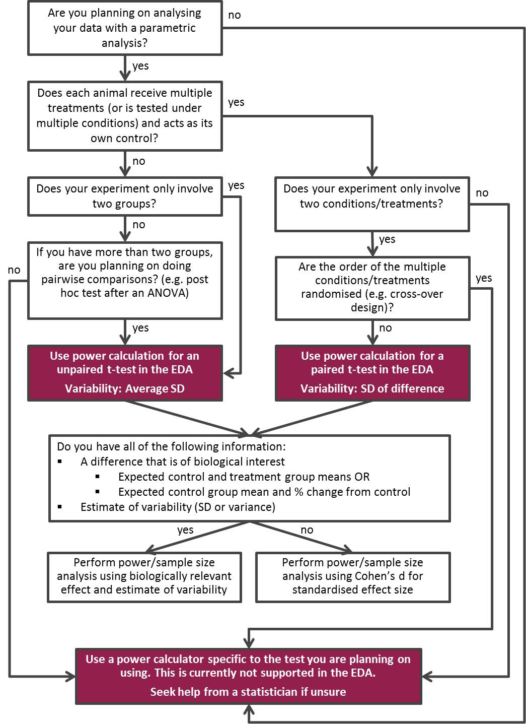
Power calculator for t-tests
Calculations for paired and unpaired t-tests can be done using the power calculator below or within the EDA. More comprehensive power analysis software is available from several sources, including Russ Lenth’s power and sample size or G Power. However, these tools should not be used without a thorough understanding of the parameters requested in the sample size computation and we recommend you seek statistical help in the first instance.
The power calculation tool below can calculate sample sizes for paired and unpaired t-tests. Use the tabs at the top of the tool to choose which calculator to use depending on your experimental design. Use the decision tree above if you need help deciding which calculator is appropriate for your experiment.
In the power calculation tool below fill out all fields except for the N per group and click Calculate. The number of experimental units per group will be displayed in the field N per group. The power calculator uses R 3.5.2 and the package power.t.test. See the section below for more information about the parameters in a power calculation for t-tests.
Parameters in a power analysis for t-tests
Sample size calculation for a t-test is based on a mathematical relationship between the following parameters: effect size, variability, significance level, power and sample size; these are described below.
Effect size (m1 – m2)
Estimating a biologically relevant effect size
The effect size is the minimum difference between two groups under study, which would be of interest biologically and would be worth taking forward into further work or clinical trials. It is based on the primary outcome measure.
You should always have an idea of what effect size would be of biological importance before carrying out an experiment. This is not based on prior knowledge of the magnitude of the treatment effect but on a difference that you want the experiment to be able to detect. In other words, the effect size is the minimum effect that you consider to be biologically important for your research question. It is not the size of effect that has been estimated or observed from experimental data in the past. Careful consideration of the effect size allows the experiment to be powered to detect only meaningful effects and not generate statistically significant results that are not biologically relevant.
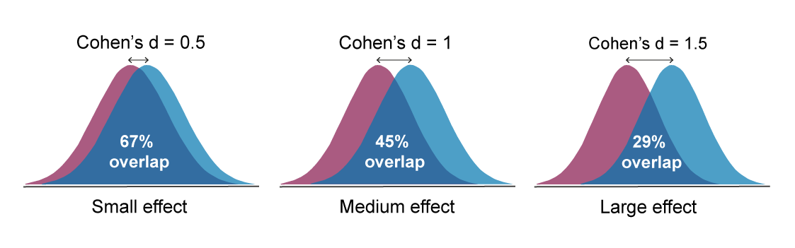
Using Cohen’s d
Cohen’s d is a standardised effect size; it represents the difference between treatment and control means, calibrated in units of variability.
Cohen's d = |m1 - m2| / average SD
A standardised effect size can be used instead of a biologically relevant one, if no information is available to estimate the variability or it is not possible to estimate the size of a biologically significant effect. Cohen’s d can be interpreted as the percentage overlap of the outcome measures in the treatment group with those of the control group.
The original guidelines suggested by Cohen in the field of social sciences suggested that small, medium and large effects were represented by d = 0.2, 0.5 and 0.8, respectively. However, in work with laboratory animals, it is generally accepted that these might more realistically be set at:
- Small effect: Cohen’s d = 0.5
- Medium effect: Cohen’s d =1.0
- Large effect: Cohen’s d =1.5
Variability (SD)
The sample size needed is related to the amount of variability between the experimental units. The larger the variability, the more animals will be required to achieve reliable results (all other things being equal). You should also consider if you are performing:
- The treatment comparison between animals, where animals are assigned to different treatment groups. In this case the power analysis for the unpaired t-test should be considered.
- The treatment comparison within-animal (i.e. each animal is used as its own control). In which case the power analysis tool for the paired t-test may be more appropriate.
Calculating estimates of variability
Calculating the average SD (standard deviation) used in the power calculation for an unpaired t-test.
There are several methods to estimate variability depending on the information available. These are listed below in order from what we believe will be the most accurate to the least accurate.
1. The most accurate estimate of variability for future studies is from data collected from a preliminary experiment carried out under identical conditions to the planned experiment (e.g. a previous experiment in the same lab, testing the same treatment, under similar conditions and on animals with the same characteristics). Such experiments are sometimes carried out to test for adverse effect or assess technical issues. Depending on the number of animals used, they can be used to estimate SD. As rule of thumb, less than 10 animals in total is unlikely to provide an accurate estimate of SD.
With two groups or more, the variability can be derived from the mean square of the residuals in an ANOVA table – the SD is calculated as the square root of this number. Alternatively, if there are only two groups the SD can be calculated as the square root of the pooled variance in a t-test table. Example SD calculations are shown in the table below.
Please note that using a covariate or a blocking factor may reduce the variability and allow the same power to be achieved with a reduced sample size. Software such as InVivoStat can be used to calculate the variability from datasets with blocking factors or covariates (using the single measure parametric analysis module). The power calculation module in InVivoStat can also be used to run the power analysis directly from a dataset.
2. If there are no data from a preliminary experiment conducted under identical conditions and the cost/benefit assessment cannot justify using extra animals for a preliminary experiment, you can consider previous experiments conducted under similar conditions in the same lab. To estimate the SD for a new experiment, you could use previous experiments which used the same animal characteristics and methods but for example tested other treatments.
As different treatments may induce different levels of variability, it is best to only consider the SD of the control group (assuming the variability is expected to be the same across all groups). This can be calculated in Excel using the function STDEV().
3. If none of the above is available (i.e. no experiment using the same type of animals in the same settings have been carried out in your lab before), it may be possible to estimate the variability from an experiment reported in the literature. Be aware that lab-to-lab differences could make this approach unreliable. If an ANOVA table is reported, it may provide an estimate of the underlying variability of the results presented – if not then the SD of the control groups can be used instead. Please note that error bars reported in the literature are not necessarily SD.
If SEM (standard error of the mean) are reported, SD can be calculated using the formula: SD = SEM × √n
If 95% CI (confidence intervals) are reported, SD can be calculated using the formula: SD = √n × (upper limit - lower limit) / 3.92
4. You may have access to a historical database of the control group data from many previous experiments (e.g. toxicity studies that have been routinely run over the years on animals with the same characteristics). Take care using this data though, as you may not have enough information about the conditions of the experiments. For example, animals may be from different batches, different suppliers or have been housed under different husbandry regimes and this may influence the underlying variability. Consider consulting a statistician before using such a database as a source of information. However, such databases do offer a large amount of information. As they will usually include data from many animals they may provide a useful estimate of the between-animal SD used in a between-animal test such as an unpaired t-test.
Calculating the SD of the differences used in the power calculation for a paired t-test.
To estimate the variability in studies where animals are used as their own control, you will need preliminary data collected under identical conditions to the planned experiment (e.g. a previous experiment in the same lab), testing the same treatment on animals with the same characteristics.
The spreadsheet below shows example calculations. Start by calculating the absolute difference between the two responses for each animal. Then the SD of these differences (across all animals) is used as the estimate of the SD within the group of animals (within-animal SD).
If variability cannot be estimated (using Cohen’s d)
Cohen’s d is a standardised effect size which is expressed in units of variability. For that reason, when Cohen’s d effect sizes are used in the t-test power calculator above (see standard effect sizes above), the variability has to be set to 1.
Significance level
The significance level or threshold (α) is the probability of obtaining a significant result by chance (a false positive) when the null hypothesis is true (i.e. there are no real, biologically relevant differences between the groups). It is usually set at 0.05 which means that the risk of obtaining a false positive is 5%; however it may be appropriate on occasion to use a different value.
Power
The power (1-β) is the probability that the experiment will correctly lead to the rejection of a false null hypothesis (i.e. detect that there is a difference when there is one). A target power between 80-95% is deemed acceptable depending on the risk of obtaining a false negative result the experimenter is willing to take.
One or two-sided test
Whether your data will be analysed using a one or two-sided test relates to whether your alternative hypothesis (H1) is directional or not. This is described in more detail on the experiment page.
If your H1 is directional (one-sided), then the experiment can be powered and analysed with a one-sided test. A directional alternative hypothesis is very rare in biology. To use one you have to accept the null hypothesis even if the results show a strong effect in the opposite direction to that set in your alternative hypothesis.
Two-sided tests with a non-directional H1 are much more common and allow you to detect the effect of a treatment regardless of its direction.
N per group
N refers to the number of experimental units needed per group, i.e. the sample size.
Representing groups in the EDA
You can represent a group of animals or experimental units in your experiment within the EDA using a group node. This can be the initial pool of animals, or a treatment or control group which has been allocated to go through a specific intervention or measurement.
In the EDA diagram, use the allocation node to indicate how you will allocate animals to groups.
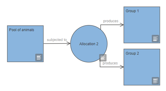
You can label group nodes to indicate what will happen to that group of animals or experimental units, or you can simply label them numerically (group 1, group 2, group 3, etc.). Every experiment should include at least one control or comparator group, and many also include a group that receives an intervention (e.g. the 'test' group). Distinct groups must have distinct labels, as the EDA will use the labels when assessing the diagram. If the same group is indicated multiple times on a diagram, it should have the exact same label each time it appears.
The properties of the group node describe the characteristics of that group, including its role in the experiment (e.g. 'test' or 'control/comparator') and details about the sample size, including justification for the sample size.
Indicating sample size in an EDA diagram
In your EDA diagram, the sample size should be indicated in the properties of the group node. The planned number of experimental units relates to the sample size you determined in the planning stages before the experiment was conducted. The sample size needs to be adjusted for potential loss of data or animals, if this is expected. A justification for the sample size (i.e. how it was determined) should also be provided. You can provide details of the power calculation used to justify your sample size – include details of the type of power calculator use and the parameters entered (effect size, variability, significance level and power).
Once the experiment has been conducted, if the actual sample size differs from the planned sample size because for example, the attrition rate was higher or lower than anticipated, the actual number of experimental units can then be indicated.
The power calculator above is also available within the EDA application as you work on your diagram. You can find it by clicking Tools in the top menu and selecting Sample Size Calculation.
References
Bate, ST (2018). How to decide your sample size when the power calculation is not straightforward.
Bate, ST and Clark, RA (2014). The Design and Statistical Analysis of Animal Experiments. Cambridge University Press.
Bate, S and Karp, NA (2014). A common control group - optimising the experiment design to maximise sensitivity. PLOS One 9(12):e114872. doi: 10.1371/journal.pone.0114872
Button, KS, et al. (2013). Power failure: why small sample size undermines the reliability of neuroscience. Nat Rev Neurosci 14(5):365-76. doi: 10.1038/nrn3475
Cohen, J (1992). A power primer. Psychol Bull 112(1):155-9. doi: 10.1037//0033-2909.112.1.155
Dell, RB, Holleran, S and Ramakrishnan, R (2002). Sample size determination. ILAR J 43(4):207-13. doi: 10.1093/ilar.43.4.207
Faul, F, et al. (2007). G*Power 3: a flexible statistical power analysis program for the social, behavioral, and biomedical sciences. Behav Res Methods 39(2):175-91. doi: 10.3758/BF03193146
Festing, MF and Altman, DG (2002). Guidelines for the design and statistical analysis of experiments using laboratory animals. ILAR J 43(4):244-58. doi: 10.1093/ilar.43.4.244
Festing, MFW, et al. (2002). The design of animal experiments: reducing the use of animals in research through better experimental design. Royal Society of Medicine.
Fitts, DA (2011). Ethics and animal numbers: informal analyses, uncertain sample sizes, inefficient replications, and type I errors. J Am Assoc Lab Anim Sci 50(4):445-53. PMID: 21838970
Fry, D (2014). Chapter 8 - Experimental Design: Reduction and Refinement in Studies Using Animals. In: Laboratory Animal Welfare (Eds. Turner, KBV). Academic Press.
Hoenig, JM and Heisey, DM (2001). The Abuse of Power. The Pervasive Fallacy of Power Calculations for Data Analysis. The American Statistician 55(1):19-24. doi: 10.1198/000313001300339897
Hubrecht, R and Kirkwood, J (2010). The UFAW handbook on the care and management of laboratory and other research animals, 8th edition. Wiley-Blackwell.
Lenth, RV (2001). Some Practical Guidelines for Effective Sample Size Determination. The American Statistician 55(3):187-193. doi: 10.1198/000313001317098149
Mead, R (1988). The design of experiments: statistical principles for practical applications. Cambridge University Press.
Reynolds PS (2019). When power calculations won’t do: Fermi approximation of animal numbers. Lab Animal. doi: 10.1038/s41684-019-0370-2
Wahlsten, D (2011). Chapter 5 - Sample Size. In: Mouse Behavioral Testing (Eds. Wahlsten, D). Academic Press.
Zakzanis, KK (2001). Statistics to tell the truth, the whole truth, and nothing but the truth: formulae, illustrative numerical examples, and heuristic interpretation of effect size analyses for neuropsychological researchers. Arch Clin Neuropsychol 16(7):653-67. PMID: 14589784